Parallel Implementation of Slice Sampling of Dirichlet Process Mixture of skew normal distributions
Source:R/DPMGibbsSkewN_parallel.R
DPMGibbsSkewN_parallel.RdIf the monitorfile argument is a character string naming a file to
write into, in the case of a new file that does not exist yet, such a new
file will be created. A line is written at each MCMC iteration.
Usage
DPMGibbsSkewN_parallel(
  Ncpus,
  type_connec,
  z,
  hyperG0,
  a = 1e-04,
  b = 1e-04,
  N,
  doPlot = FALSE,
  nbclust_init = 30,
  plotevery = N/10,
  diagVar = TRUE,
  use_variance_hyperprior = TRUE,
  verbose = FALSE,
  monitorfile = "",
  ...
)
Arguments
- Ncpus
the number of processors available
- type_connec
The type of connection between the processors. Supported cluster types are
"SOCK","FORK","MPI", and"NWS". See alsomakeCluster.- z
data matrix
d x nwithddimensions in rows andnobservations in columns.- hyperG0
prior mixing distribution.
- a
shape hyperparameter of the Gamma prior on the concentration parameter of the Dirichlet Process. Default is
0.0001.- b
scale hyperparameter of the Gamma prior on the concentration parameter of the Dirichlet Process. Default is
0.0001. If0, then the concentration is fixed set toa.- N
number of MCMC iterations.
- doPlot
logical flag indicating whether to plot MCMC iteration or not. Default to
TRUE.- nbclust_init
number of clusters at initialization. Default to 30 (or less if there are less than 30 observations).
- plotevery
an integer indicating the interval between plotted iterations when
doPlotisTRUE.- diagVar
logical flag indicating whether the variance of each cluster is estimated as a diagonal matrix, or as a full matrix. Default is
TRUE(diagonal variance).- use_variance_hyperprior
logical flag indicating whether a hyperprior is added for the variance parameter. Default is
TRUEwhich decrease the impact of the variance prior on the posterior.FALSEis useful for using an informative prior.- verbose
logical flag indicating whether partition info is written in the console at each MCMC iteration.
- monitorfile
a writable connections or a character string naming a file to write into, to monitor the progress of the analysis. Default is
""which is no monitoring. See Details.- ...
additional arguments to be passed to
plot_DPM. Only used ifdoPlotisTRUE.
Value
a object of class DPMclust with the following attributes:
mcmc_partitions:a list of length
N. Each elementmcmc_partitions[n]is a vector of lengthngiving the partition of thenobservations.alpha:a vector of length
N.cost[j]is the cost associated to partitionc[[j]]U_SS_list:a list of length
Ncontaining the lists of sufficient statistics for all the mixture components at each MCMC iterationweights_list:logposterior_list:a list of length
Ncontaining the logposterior values at each MCMC iterationsdata:the data matrix
d x nwithddimensions in rows andnobservations in columnsnb_mcmcit:the number of MCMC iterations
clust_distrib:the parametric distribution of the mixture component -
"skewnorm"hyperG0:the prior on the cluster location
References
Hejblum BP, Alkhassim C, Gottardo R, Caron F and Thiebaut R (2019) Sequential Dirichlet Process Mixtures of Multivariate Skew t-distributions for Model-based Clustering of Flow Cytometry Data. The Annals of Applied Statistics, 13(1): 638-660. <doi: 10.1214/18-AOAS1209> <arXiv: 1702.04407> https://arxiv.org/abs/1702.04407 doi:10.1214/18-AOAS1209
Examples
rm(list=ls())
#Number of data
n <- 2000
set.seed(1234)
d <- 4
ncl <- 5
# Sample data
sdev <- array(dim=c(d,d,ncl))
xi <- matrix(nrow=d, ncol=ncl, c(runif(n=d*ncl,min=0,max=3)))
psi <- matrix(nrow=d, ncol=ncl, c(runif(n=d*ncl,min=-1,max=1)))
p <- runif(n=ncl)
p <- p/sum(p)
sdev0 <- diag(runif(n=d, min=0.05, max=0.6))
for (j in 1:ncl){
sdev[, ,j] <- invwishrnd(n = d+2, lambda = sdev0)
}
c <- rep(0,n)
z <- matrix(0, nrow=d, ncol=n)
for(k in 1:n){
c[k] = which(rmultinom(n=1, size=1, prob=p)!=0)
z[,k] <- xi[, c[k]] + psi[, c[k]]*abs(rnorm(1)) + sdev[, , c[k]]%*%matrix(rnorm(d, mean = 0,
sd = 1), nrow=d, ncol=1)
#cat(k, "/", n, " observations simulated\n", sep="")
}
# Set parameters of G0
hyperG0 <- list()
hyperG0[["b_xi"]] <- rep(0,d)
hyperG0[["b_psi"]] <- rep(0,d)
hyperG0[["kappa"]] <- 0.001
hyperG0[["D_xi"]] <- 100
hyperG0[["D_psi"]] <- 100
hyperG0[["nu"]] <- d + 1
hyperG0[["lambda"]] <- diag(d)/10
# hyperprior on the Scale parameter of DPM
a <- 0.0001
b <- 0.0001
# do some plots
doPlot <- TRUE
nbclust_init <- 30
z <- z*200
## Data
########
library(ggplot2)
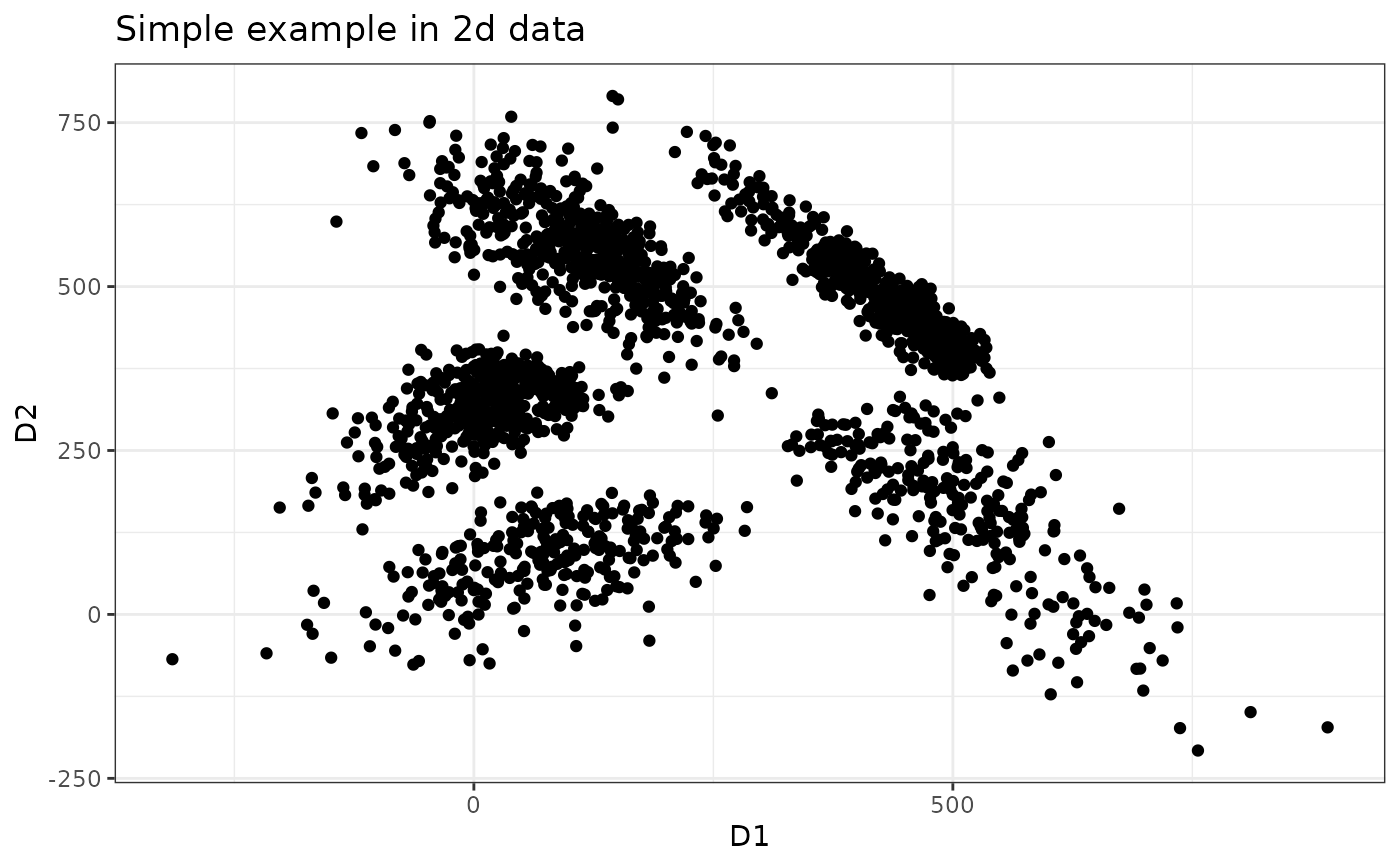
p <- (ggplot(data.frame("X"=z[1,], "Y"=z[2,]), aes(x=X, y=Y))
+ geom_point()
+ ggtitle("Simple example in 2d data")
+xlab("D1")
+ylab("D2")
+theme_bw())
p
 ## alpha priors plots
#####################
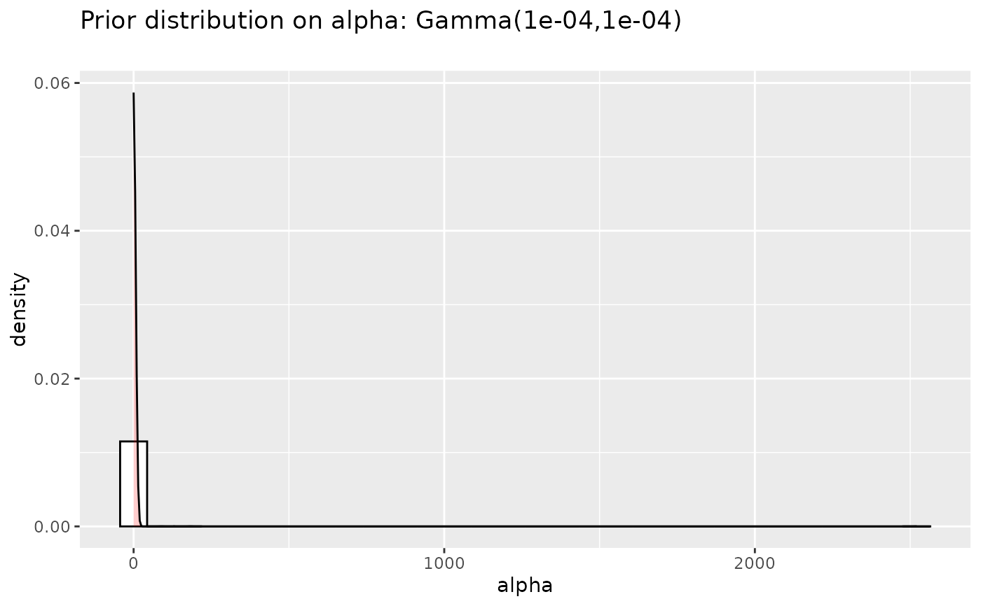
prioralpha <- data.frame("alpha"=rgamma(n=5000, shape=a, scale=1/b),
"distribution" =factor(rep("prior",5000),
levels=c("prior", "posterior")))
p <- (ggplot(prioralpha, aes(x=alpha))
+ geom_histogram(aes(y=..density..),
colour="black", fill="white")
+ geom_density(alpha=.2, fill="red")
+ ggtitle(paste("Prior distribution on alpha: Gamma(", a,
",", b, ")\n", sep=""))
)
p
#> `stat_bin()` using `bins = 30`. Pick better value `binwidth`.
## alpha priors plots
#####################
prioralpha <- data.frame("alpha"=rgamma(n=5000, shape=a, scale=1/b),
"distribution" =factor(rep("prior",5000),
levels=c("prior", "posterior")))
p <- (ggplot(prioralpha, aes(x=alpha))
+ geom_histogram(aes(y=..density..),
colour="black", fill="white")
+ geom_density(alpha=.2, fill="red")
+ ggtitle(paste("Prior distribution on alpha: Gamma(", a,
",", b, ")\n", sep=""))
)
p
#> `stat_bin()` using `bins = 30`. Pick better value `binwidth`.
 # Gibbs sampler for Dirichlet Process Mixtures
##############################################
if(interactive()){
MCMCsample_sn_par <- DPMGibbsSkewN_parallel(Ncpus=parallel::detectCores()-1,
type_connec="SOCK", z, hyperG0,
a, b, N=5000, doPlot, nbclust_init,
plotevery=25, gg.add=list(theme_bw(),
guides(shape=guide_legend(override.aes = list(fill="grey45")))))
plot_ConvDPM(MCMCsample_sn_par, from=2)
}
# Gibbs sampler for Dirichlet Process Mixtures
##############################################
if(interactive()){
MCMCsample_sn_par <- DPMGibbsSkewN_parallel(Ncpus=parallel::detectCores()-1,
type_connec="SOCK", z, hyperG0,
a, b, N=5000, doPlot, nbclust_init,
plotevery=25, gg.add=list(theme_bw(),
guides(shape=guide_legend(override.aes = list(fill="grey45")))))
plot_ConvDPM(MCMCsample_sn_par, from=2)
}