Slice Sampling of Dirichlet Process Mixture of skew Student's t-distributions
Source:R/DPMGibbsSkewT.R
DPMGibbsSkewT.RdSlice Sampling of Dirichlet Process Mixture of skew Student's t-distributions
Usage
DPMGibbsSkewT(
  z,
  hyperG0,
  a = 1e-04,
  b = 1e-04,
  N,
  doPlot = TRUE,
  nbclust_init = 30,
  plotevery = N/10,
  diagVar = TRUE,
  use_variance_hyperprior = TRUE,
  verbose = TRUE,
  ...
)
Arguments
- z
data matrix
d x nwithddimensions in rows andnobservations in columns.- hyperG0
parameters of the prior mixing distribution in a
listwith the following named components:"b_xi": a vector of lengthdwith the mean location prior parameter. Can be set as the empirical mean of the data in an Empirical Bayes fashion."b_psi": a vector of lengthdwith the skewness location prior parameter. Can be set as 0 a priori."kappa": a strictly positive number part of the inverse-Wishart component of the prior on the variance matrix. Can be set as very small (e.g. 0.001) a priori."D_xi": hyperprior controlling the information in \(\xi\) (the larger the less information is carried). 100 is a reasonable value, based on Fruhwirth-Schnatter et al., Biostatistics, 2010."D_psi": hyperprior controlling the information in \(\psi\) (the larger the less information is carried). 100 is a reasonable value, based on Fruhwirth-Schnatter et al., Biostatistics, 2010"nu": a prior number on the degrees of freedom of the \(t\) component that must be strictly greater thand. Can be set asd + 1for instance."lambda": ad x dsymmetric definitive positive matrix part of the inverse-Wishart component of the prior on the variance matrix. Can be set as the diagonal of empirical variance of the data in an Empircal Bayes fashion divided by a factor 3 according to Fruhwirth-Schnatter et al., Biostatistics, 2010.
- a
shape hyperparameter of the Gamma prior on the concentration parameter of the Dirichlet Process. Default is
0.0001.- b
scale hyperparameter of the Gamma prior on the concentration parameter of the Dirichlet Process. Default is
0.0001. If0, then the concentration is fixed set toa.- N
number of MCMC iterations.
- doPlot
logical flag indicating whether to plot MCMC iteration or not. Default to
TRUE.- nbclust_init
number of clusters at initialization. Default to 30 (or less if there are less than 30 observations).
- plotevery
an integer indicating the interval between plotted iterations when
doPlotisTRUE.- diagVar
logical flag indicating whether the variance of each cluster is estimated as a diagonal matrix, or as a full matrix. Default is
TRUE(diagonal variance).- use_variance_hyperprior
logical flag indicating whether a hyperprior is added for the variance parameter. Default is
TRUEwhich decrease the impact of the variance prior on the posterior.FALSEis useful for using an informative prior.- verbose
logical flag indicating whether partition info is written in the console at each MCMC iteration.
- ...
additional arguments to be passed to
plot_DPMst. Only used ifdoPlotisTRUE.
Value
a object of class DPMclust with the following attributes:
mcmc_partitions:a list of length
N. Each elementmcmc_partitions[n]is a vector of lengthngiving the partition of thenobservations.alpha:a vector of length
N.cost[j]is the cost associated to partitionc[[j]]U_SS_list:a list of length
Ncontaining the lists of sufficient statistics for all the mixture components at each MCMC iterationweights_list:a list of length
Ncontaining the weights of each mixture component for each MCMC iterationslogposterior_list:a list of length
Ncontaining the logposterior values at each MCMC iterationsdata:the data matrix
d x nwithddimensions in rows andnobservations in columnsnb_mcmcit:the number of MCMC iterations
clust_distrib:the parametric distribution of the mixture component -
"skewt"hyperG0:the prior on the cluster location
References
Hejblum BP, Alkhassim C, Gottardo R, Caron F and Thiebaut R (2019) Sequential Dirichlet Process Mixtures of Multivariate Skew t-distributions for Model-based Clustering of Flow Cytometry Data. The Annals of Applied Statistics, 13(1): 638-660. <doi: 10.1214/18-AOAS1209> <arXiv: 1702.04407> https://arxiv.org/abs/1702.04407 doi:10.1214/18-AOAS1209
Fruhwirth-Schnatter S, Pyne S, Bayesian inference for finite mixtures of univariate and multivariate skew-normal and skew-t distributions, Biostatistics, 2010.
Examples
rm(list=ls())
#Number of data
n <- 2000
set.seed(4321)
d <- 2
ncl <- 4
# Sample data
library(truncnorm)
sdev <- array(dim=c(d,d,ncl))
#xi <- matrix(nrow=d, ncol=ncl, c(-1.5, 1.5, 1.5, 1.5, 2, -2.5, -2.5, -3))
#xi <- matrix(nrow=d, ncol=ncl, c(-0.5, 0, 0.5, 0, 0.5, -1, -1, 1))
xi <- matrix(nrow=d, ncol=ncl, c(-0.2, 0.5, 2.4, 0.4, 0.6, -1.3, -0.9, -2.7))
psi <- matrix(nrow=d, ncol=4, c(0.3, -0.7, -0.8, 0, 0.3, -0.7, 0.2, 0.9))
nu <- c(100,25,8,5)
p <- c(0.15, 0.05, 0.5, 0.3) # frequence des clusters
sdev[, ,1] <- matrix(nrow=d, ncol=d, c(0.3, 0, 0, 0.3))
sdev[, ,2] <- matrix(nrow=d, ncol=d, c(0.1, 0, 0, 0.3))
sdev[, ,3] <- matrix(nrow=d, ncol=d, c(0.3, 0.15, 0.15, 0.3))
sdev[, ,4] <- .3*diag(2)
c <- rep(0,n)
w <- rep(1,n)
z <- matrix(0, nrow=d, ncol=n)
for(k in 1:n){
c[k] = which(rmultinom(n=1, size=1, prob=p)!=0)
w[k] <- rgamma(1, shape=nu[c[k]]/2, rate=nu[c[k]]/2)
z[,k] <- xi[, c[k]] + psi[, c[k]]*rtruncnorm(n=1, a=0, b=Inf, mean=0, sd=1/sqrt(w[k])) +
(sdev[, , c[k]]/sqrt(w[k]))%*%matrix(rnorm(d, mean = 0, sd = 1), nrow=d, ncol=1)
#cat(k, "/", n, " observations simulated\n", sep="")
}
# Set parameters of G0
hyperG0 <- list()
hyperG0[["b_xi"]] <- rowMeans(z)
hyperG0[["b_psi"]] <- rep(0,d)
hyperG0[["kappa"]] <- 0.001
hyperG0[["D_xi"]] <- 100
hyperG0[["D_psi"]] <- 100
hyperG0[["nu"]] <- d+1
hyperG0[["lambda"]] <- diag(apply(z,MARGIN=1, FUN=var))/3
# hyperprior on the Scale parameter of DPM
a <- 0.0001
b <- 0.0001
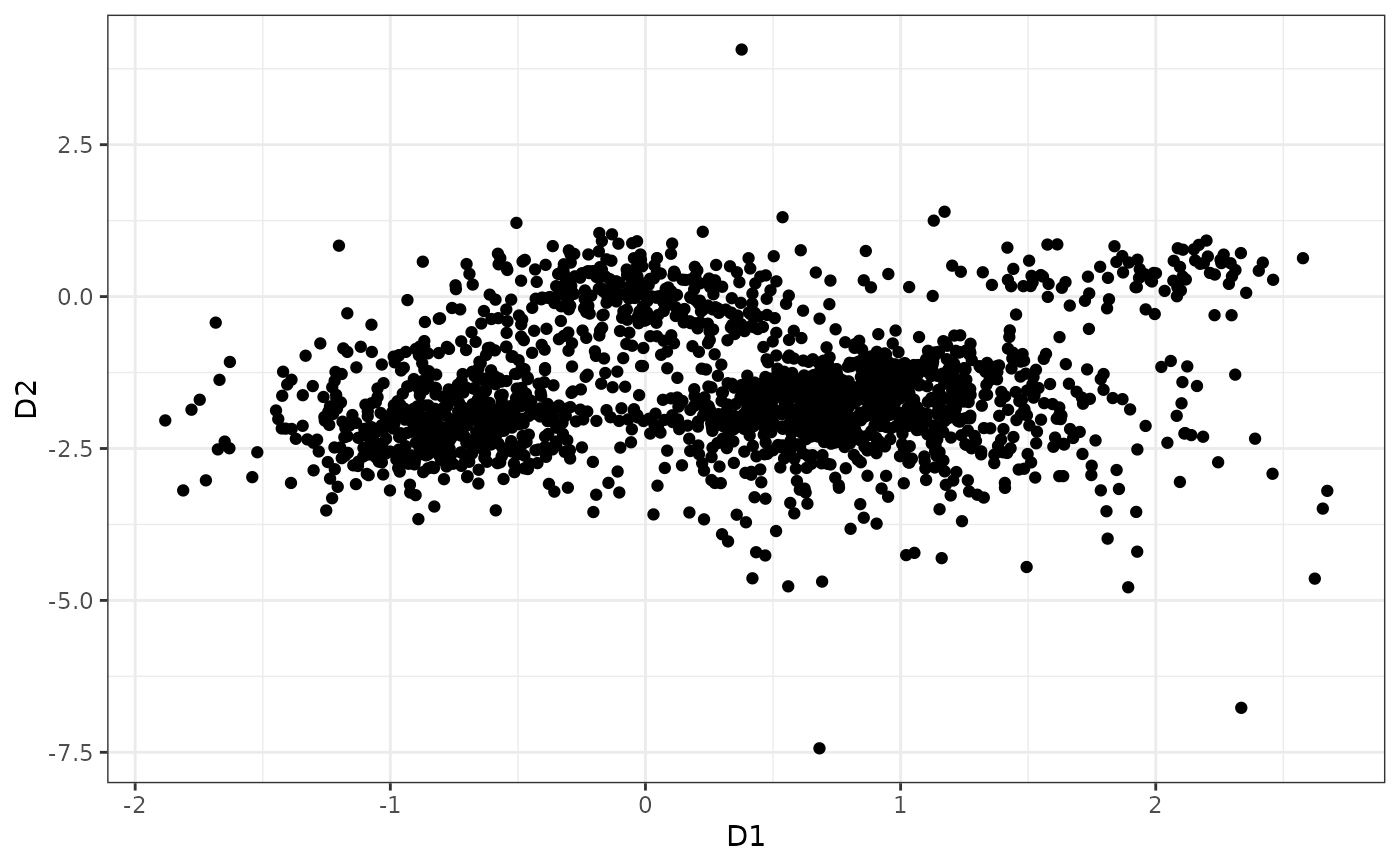
## Data
########
library(ggplot2)
p <- (ggplot(data.frame("X"=z[1,], "Y"=z[2,]), aes(x=X, y=Y))
+ geom_point()
#+ ggtitle("Simple example in 2d data")
+xlab("D1")
+ylab("D2")
+theme_bw())
p #pdf(height=8.5, width=8.5)
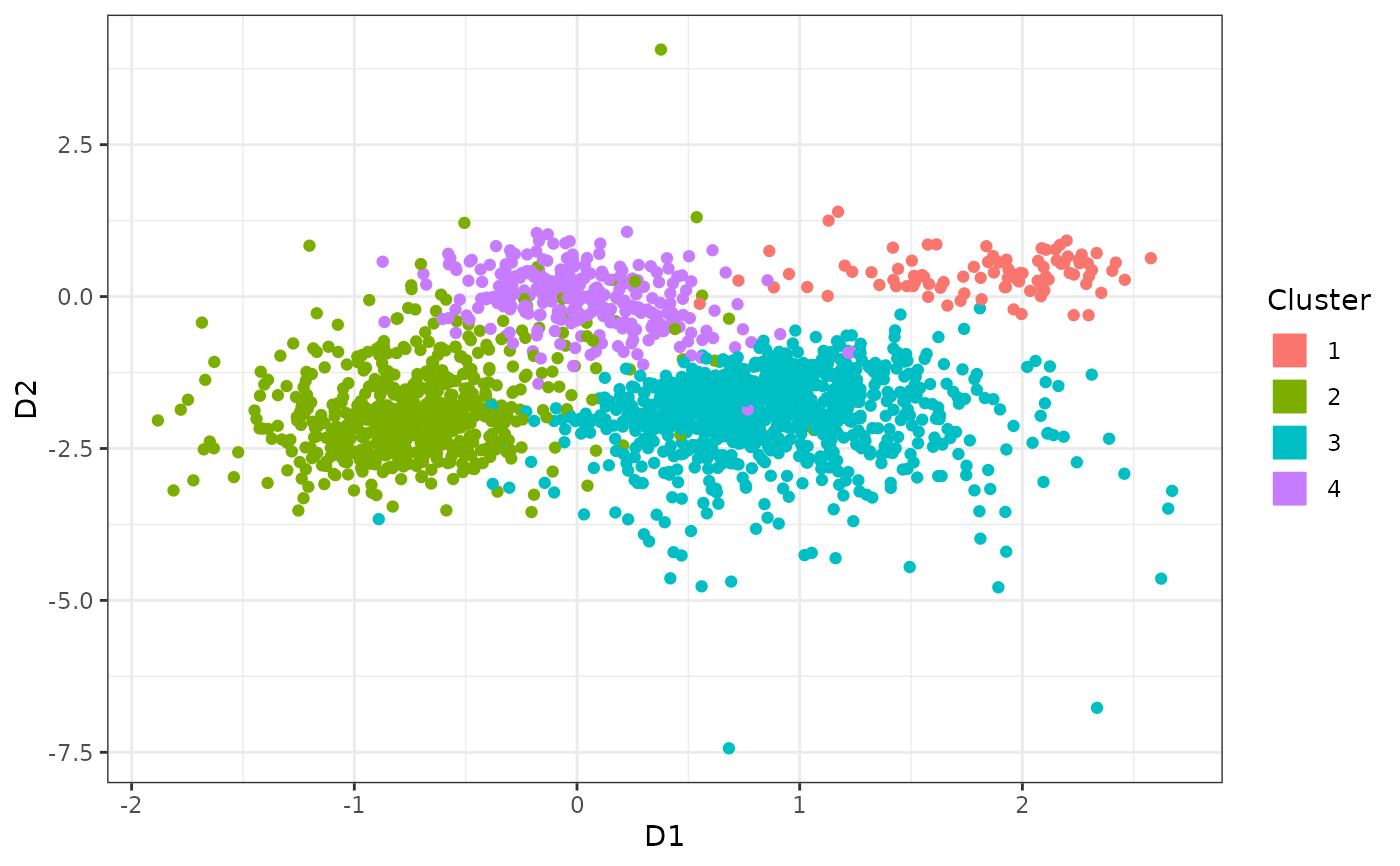
 c2plot <- factor(c)
levels(c2plot) <- c("4", "1", "3", "2")
pp <- (ggplot(data.frame("X"=z[1,], "Y"=z[2,], "Cluster"=as.character(c2plot)))
+ geom_point(aes(x=X, y=Y, colour=Cluster, fill=Cluster))
#+ ggtitle("Slightly overlapping skew-normal simulation\n")
+ xlab("D1")
+ ylab("D2")
+ theme_bw()
+ scale_colour_discrete(guide=guide_legend(override.aes = list(size = 6, shape=22))))
pp #pdf(height=7, width=7.5)
c2plot <- factor(c)
levels(c2plot) <- c("4", "1", "3", "2")
pp <- (ggplot(data.frame("X"=z[1,], "Y"=z[2,], "Cluster"=as.character(c2plot)))
+ geom_point(aes(x=X, y=Y, colour=Cluster, fill=Cluster))
#+ ggtitle("Slightly overlapping skew-normal simulation\n")
+ xlab("D1")
+ ylab("D2")
+ theme_bw()
+ scale_colour_discrete(guide=guide_legend(override.aes = list(size = 6, shape=22))))
pp #pdf(height=7, width=7.5)
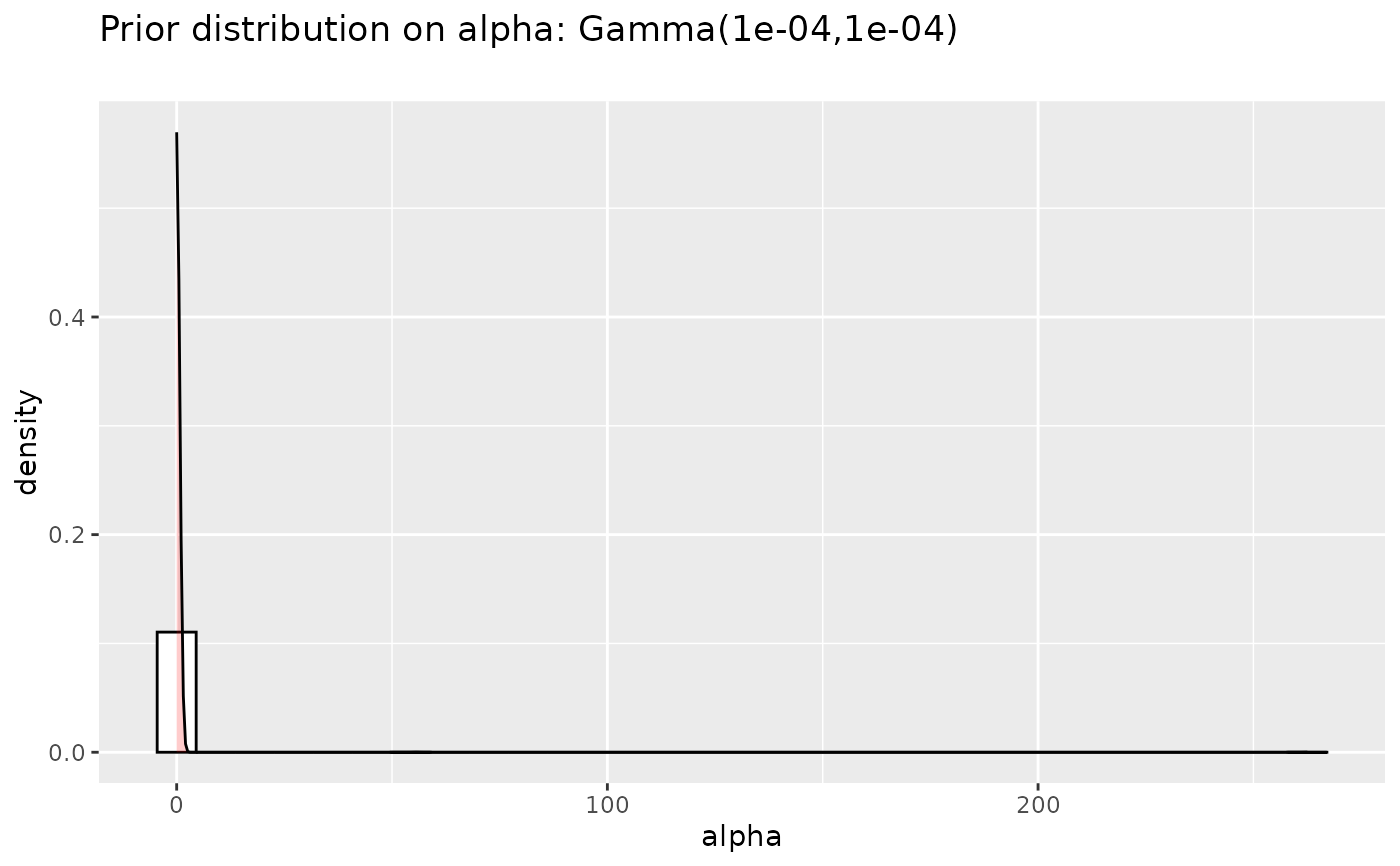
 ## alpha priors plots
#####################
prioralpha <- data.frame("alpha"=rgamma(n=5000, shape=a, scale=1/b),
"distribution" =factor(rep("prior",5000),
levels=c("prior", "posterior")))
p <- (ggplot(prioralpha, aes(x=alpha))
+ geom_histogram(aes(y=..density..),
colour="black", fill="white")
+ geom_density(alpha=.2, fill="red")
+ ggtitle(paste("Prior distribution on alpha: Gamma(", a,
",", b, ")\n", sep=""))
)
p
#> `stat_bin()` using `bins = 30`. Pick better value `binwidth`.
## alpha priors plots
#####################
prioralpha <- data.frame("alpha"=rgamma(n=5000, shape=a, scale=1/b),
"distribution" =factor(rep("prior",5000),
levels=c("prior", "posterior")))
p <- (ggplot(prioralpha, aes(x=alpha))
+ geom_histogram(aes(y=..density..),
colour="black", fill="white")
+ geom_density(alpha=.2, fill="red")
+ ggtitle(paste("Prior distribution on alpha: Gamma(", a,
",", b, ")\n", sep=""))
)
p
#> `stat_bin()` using `bins = 30`. Pick better value `binwidth`.
 if(interactive()){
# Gibbs sampler for Dirichlet Process Mixtures
##############################################
MCMCsample_st <- DPMGibbsSkewT(z, hyperG0, a, b, N=1500,
doPlot=TRUE, nbclust_init=30, plotevery=100,
diagVar=FALSE)
s <- summary(MCMCsample_st, burnin = 1000, thin=10, lossFn = "Binder")
print(s)
plot(s, hm=TRUE) #pdf(height=8.5, width=10.5) #png(height=700, width=720)
plot_ConvDPM(MCMCsample_st, from=2)
#cluster_est_binder(MCMCsample_st$mcmc_partitions[900:1000])
}
if(interactive()){
# Gibbs sampler for Dirichlet Process Mixtures
##############################################
MCMCsample_st <- DPMGibbsSkewT(z, hyperG0, a, b, N=1500,
doPlot=TRUE, nbclust_init=30, plotevery=100,
diagVar=FALSE)
s <- summary(MCMCsample_st, burnin = 1000, thin=10, lossFn = "Binder")
print(s)
plot(s, hm=TRUE) #pdf(height=8.5, width=10.5) #png(height=700, width=720)
plot_ConvDPM(MCMCsample_st, from=2)
#cluster_est_binder(MCMCsample_st$mcmc_partitions[900:1000])
}