Sampler for the concentration parameter of a Dirichlet process

Sampler updating the concentration parameter of a Dirichlet process given the number of observations and a Gamma(a, b) prior, following the augmentation strategy of West, and of Escobar and West.

Usage

sample_alpha(alpha_old, n, K, a = 1e-04, b = 1e-04)

Arguments

alpha_old: the current value of alpha
n: the number of data points
K: current number of cluster
a: shape hyperparameter of the Gamma prior on the concentration parameter of the Dirichlet Process. Default is 0.0001.
b: scale hyperparameter of the Gamma prior on the concentration parameter of the Dirichlet Process. Default is 0.0001. If 0 then the concentration is fixed and this function returns a.

Details

A Gamma prior is used.

References

M West, Hyperparameter estimation in Dirichlet process mixture models, Technical Report, Duke University, 1992.

MD Escobar, M West, Bayesian Density Estimation and Inference Using Mixtures Journal of the American Statistical Association, 90(430):577-588, 1995.

Examples

#Test with a fixed K
####################

alpha_init <- 1000
N <- 10000
#n=500
n=10000
K <- 80
a <- 0.0001
b <- a
alphas <- numeric(N)
alphas[1] <- alpha_init
for (i in 2:N){
 alphas[i] <- sample_alpha(alpha_old = alphas[i-1], n=n, K=K, a=a, b=b)
}

postalphas <- alphas[floor(N/2):N]
alphaMMSE <- mean(postalphas)
alphaMAP <- density(postalphas)$x[which.max(density(postalphas)$y)]

expK <- sum(alphaMMSE/(alphaMMSE+0:(n-1)))
round(expK)
#> [1] 80


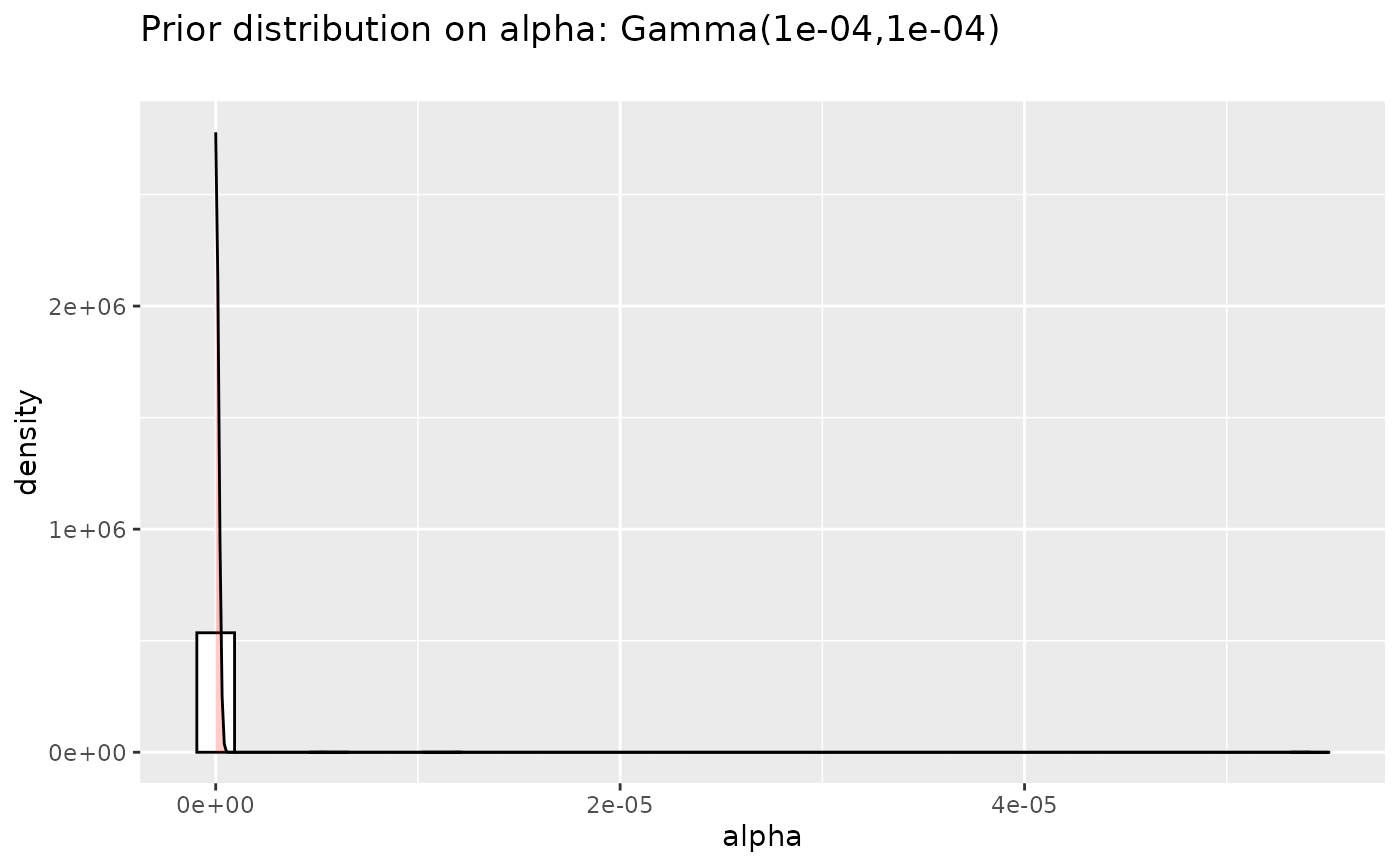
 prioralpha <- data.frame("alpha"=rgamma(n=5000, a,1/b),
                         "distribution" =factor(rep("prior",5000),
                         levels=c("prior", "posterior")))

 library(ggplot2)
 p <- (ggplot(prioralpha, aes(x=alpha))
       + geom_histogram(aes(y=..density..),
                        colour="black", fill="white")
       + geom_density(alpha=.2, fill="red")
       + ggtitle(paste("Prior distribution on alpha: Gamma(", a,
                 ",", b, ")\n", sep=""))
      )
 p
#> `stat_bin()` using `bins = 30`. Pick better value with `binwidth`.


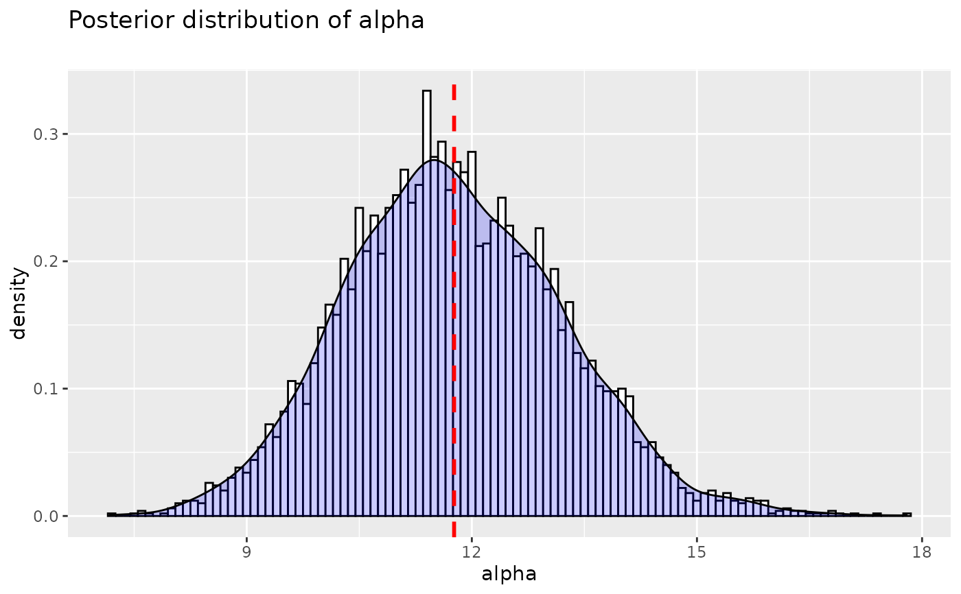
postalpha.df <- data.frame("alpha"=postalphas,
                         "distribution" = factor(rep("posterior",length(postalphas)),
                         levels=c("prior", "posterior")))
 p <- (ggplot(postalpha.df, aes(x=alpha))
       + geom_histogram(aes(y=..density..), binwidth=.1,
                        colour="black", fill="white")
       + geom_density(alpha=.2, fill="blue")
       + ggtitle("Posterior distribution of alpha\n")
       # Ignore NA values for mean
       # Overlay with transparent density plot
       + geom_vline(aes(xintercept=mean(alpha, na.rm=TRUE)),
                    color="red", linetype="dashed", size=1)
     )
#> Warning: Using `size` aesthetic for lines was deprecated in ggplot2 3.4.0.
#> ℹ Please use `linewidth` instead.
 p