User guide to the citcdf R package

1 Overview of `citcdf`

citcdf performs conditional independence testing through conditional cumulative distribution functions (Gauthier et al. 2021). It addresses the following null hypothesis: $H_0: Y \perp\!\!\!\perp X \mid Z$

by testing whether $F_{Y \mid X, Z}(y) = F_{Y \mid Z}(y)$ . The associated test statistic is computed across a grid of thresholds $\omega_1 < \dots < \omega_p$ spanning $Y$ , where the indicator $\mathbb{1}_{Y_i \le \omega_j}$ is regressed on both $X$ and $Z$ at each threshold $j$ . Under $H_0$ , the coefficients $\beta_j$ carried by $X$ are all null, and thus citcdf test statistic is the sum of squares whose asymptotic distribution is then a weighted mixture of $\chi^2_1$ .

No distributional assumption is made on $Y$ , and in that sense citcdf is distribution-free. It is therefore robust to zero-inflation, multi-modality and skewness that typical occur in single-cell RNA-seq data.

1.1 Main user functions

Three main functions build form the citcdfpackage leverage this test statistic:

cit_asymp(): one hypothesis, asymptotic p-value
cit_perm(): one hypothesis, permutation p-value
cit_multi(): many outcomes at once (with a Benjamini-Hochberg adjustment), either asymptotic or permutation test

1.2 Inputs

Y is a numeric vector. X and Z are data frames, one column per variable, numeric or factor. Gene set analysis is available through cit_gsa() and is not covered here.

library(citcdf)
set.seed(20260817)

2 Testing a single hypothesis

2.1 The data

We use the marksdataset, from the bnlearn package (Scutari 2010). It records the exam marks of 88 students in five mathematics topics (Mardia et al. 1979). Of note, mechanics and statistics marks are correlated, but the association is mediated by the algebra mark (relevant to both disciplines).

data("marks", package = "bnlearn")
str(marks)
#> 'data.frame':    88 obs. of  5 variables:
#>  $ MECH: num  77 63 75 55 63 53 51 59 62 64 ...
#>  $ VECT: num  82 78 73 72 63 61 67 70 60 72 ...
#>  $ ALG : num  67 80 71 63 65 72 65 68 58 60 ...
#>  $ ANL : num  67 70 66 70 70 64 65 62 62 62 ...
#>  $ STAT: num  81 81 81 68 63 73 68 56 70 45 ...

2.2 Asymptotic test with `cit_asymp()`

$Y$ is the statistics mark, $X$ the mechanics mark. Without conditioning:

Y <- marks$STAT
X <- data.frame(MECH = marks$MECH)

cit_asymp(Y, X)
#>       raw_pval test_statistic
#> 1 0.0003640664      0.1797552

Conditioning on the algebra mark asks whether mechanics adds anything beyond algebra:

Z <- data.frame(ALG = marks$ALG)

cit_asymp(Y, X, Z)
#>    raw_pval test_statistic
#> 1 0.6204986     0.01850231

The evidence disappears.

NB: cit_asymp() assumed neither normality nor linearity.
It remains valid for skewed, zero-inflated or multi-modal outcomes.

Of note, bnlearn::ci.test() reaches the same conclusion from a Gaussian correlation statistic:

bnlearn::ci.test("STAT", "MECH", data = marks, test = "cor")$p.value
#> [1] 0.0001792015
bnlearn::ci.test("STAT", "MECH", "ALG", data = marks, test = "cor")$p.value
#> [1] 0.7060518

2.3 Permutation test with `cit_perm()`

The asymptotic null distribution requires a reasonable sample size. For small n, cit_perm() calibrates the same observed statistic against a permutation null:

cit_perm(Y, X, n_perm = 1000)
#>   score    raw_pval test_statistic
#> 1     0 0.000999001      0.1797552

test_statistic remains identical to the one returned by cit_asymp(), and score counts the permutations reaching the observed statistic: the (unbiased) permutation p-value is then computed as (score + 1) / (n_perm + 1) (so n_perm also fixes the smallest reachable p-value, ie. 1/(n_perm +1).

Permuting $X$ freely would destroy its association with $Z$ and test the wrong null. X_perm() computes design permutations conditionally on $Z$ :

$Z$ discrete: permutes within each strata of $Z$
$Z$ continuous: permutes by matching observations on the fitted value of $X$ given $Z$ , following Berrett et al. (2020) (see ?perm_cont)

cit_perm(Y, X, Z = Z, n_perm = 1000)
#>   score  raw_pval test_statistic
#> 1   523 0.5234765     0.01850231

Both tests agree on both hypotheses.

NB: cit_perm() only accepts a single covariate column when Z is not NULL. Multiple X with Z present require the asymptotic test.

2.4 Visualization

plot_compare_ccdf() displays what the statistic compares: the CCDF of $Y$ given $X$ against its marginal counterpart. The further apart the 2 are, the larger $D$ :

plot_compare_ccdf(Y = data.frame(STAT = Y), X = X)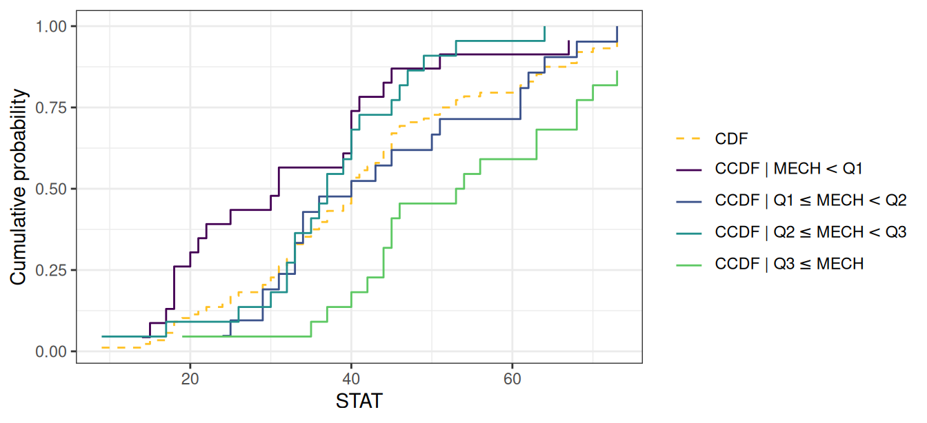

3 Testing many outcomes with `cit_multi()`

cit_multi() loops the test over the columns of a matrix M of n observations by r outcomes, and returns Benjamini-Hochberg adjusted p-values (alongside the raw ones).

3.1 scRNA-seq data

This vignette uses pbmc_small, the PBMC scRNA-seq excerpt distributed with the SeuratObject package (Satija et al. 2023) (230 genes, 80 cells).

NB: M must be oriented cells-by-genes, the transpose of usual genes-by-cells expression matrix. Also, outcomes with no variability must be filtered-out beforehand (otherwise an error is triggered).

data("pbmc_small", package = "SeuratObject")
expr <- as.matrix(SeuratObject::LayerData(pbmc_small, layer = "data"))
cell_md <- pbmc_small[[]]

expr <- expr[apply(expr, 1, function(g) length(unique(g)) > 1), ]
M <- as.data.frame(t(expr))
dim(M)
#> [1]  80 230

The variable of interest is the cell population (letter.idents, two populations). The two populations were not sequenced to comparable depth:

tapply(cell_md$nCount_RNA, cell_md$letter.idents, median)
#>   A   B 
#> 150 353

Library size is therefore a candidate confounder. An unadjusted comparison will identify significant genes that are only associated with sequencing depth.

3.2 Asymptotic analysis

X_pop <- data.frame(pop = cell_md$letter.idents)
Z_lib <- data.frame(libsize = cell_md$nCount_RNA)

res_unadj <- cit_multi(M, X = X_pop, test = "asymptotic", parallel = FALSE)
res_adj <- cit_multi(M, X = X_pop, Z = Z_lib, test = "asymptotic",
                     parallel = FALSE)

c(unadjusted = sum(res_unadj$pvals$adj_pval < 0.05),
  adjusted   = sum(res_adj$pvals$adj_pval < 0.05))
#> unadjusted   adjusted 
#>         89         55

Conditioning on library size withdraws a third of the hits. The strongest signals — canonical monocyte markers — survive:

head(res_adj$pvals[order(res_adj$pvals$raw_pval), ], 5)
#>            raw_pval     adj_pval test_statistic
#> S100A8 1.951411e-11 4.488246e-09       246.5594
#> S100A9 7.526161e-11 8.655085e-09       250.5153
#> TYMP   3.219987e-08 2.468657e-06       256.8253
#> AIF1   9.697369e-08 5.430011e-06       205.6298
#> IFITM3 1.180437e-07 5.430011e-06       195.7231

res_adj is a list containing:

which_test and n_perm, the test performed and the number of permutations (NA for the asymptotic test)
pvals, the gene-wise raw and BH-adjusted p-values, plus the test statistics

The plot() method sorts the raw p-values against the BH threshold and the nominal level:

plot(res_adj)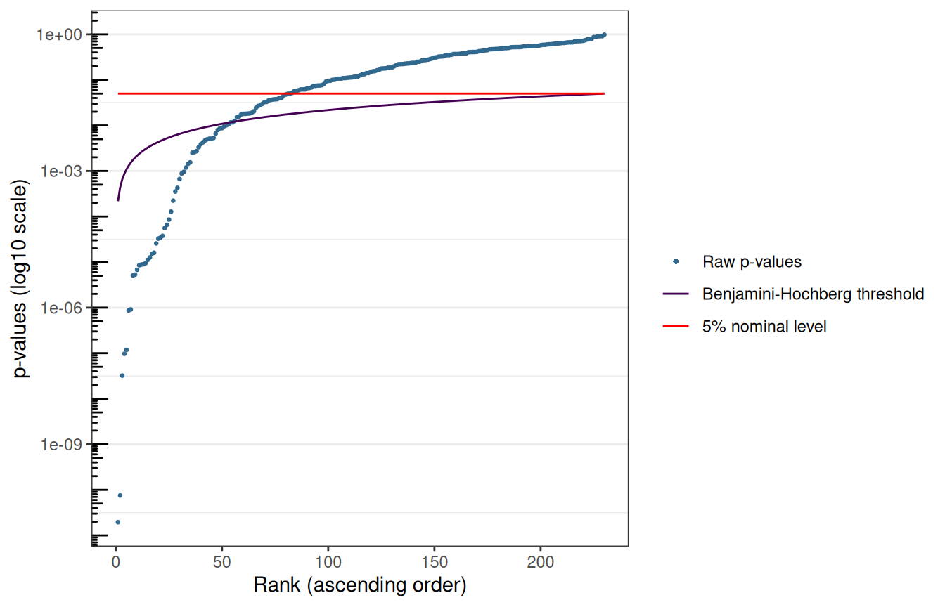

3.3 Visualization

plot_compare_ccdf() details one gene. Panel A contrasts the CCDF given the cell population with the marginal CDF. Panel B repeats the comparison within library-size quartiles.

top_gene <- rownames(res_adj$pvals)[which.min(res_adj$pvals$raw_pval)]
plot_compare_ccdf(Y = M[, top_gene, drop = FALSE], X = X_pop, Z = Z_lib,
                  space_y = TRUE, number_y = 20)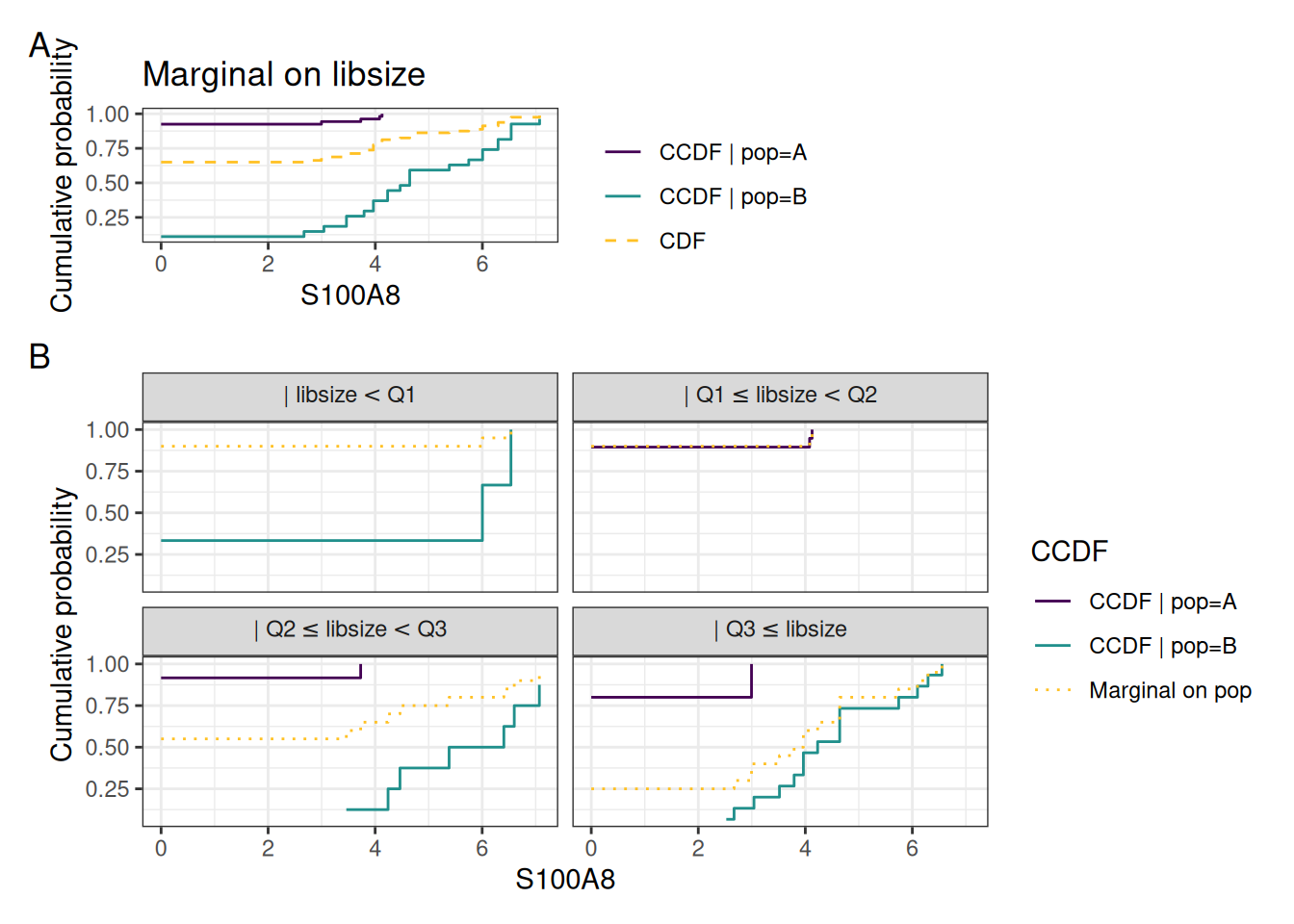

3.4 Permutation analysis

With 80 cells, the asymptotic approximation should work (low end of its range). test = "permutation" confirms a few genes. adaptive = TRUE (the default) spends additional computation time to increase p-value resolution where it matters (especially for FDR-adjusted p-values): all outcomes start at n_perm, and only those still significant proceed to the larger stages of n_perm_adaptive.

res_perm <- cit_multi(M, X = X_pop, Z = Z_lib, test = "permutation",
                      n_perm = 100, parallel = FALSE)
#> Computing 100 permutations...
#> Computing 100 additional permutations...
#> Computing 300 additional permutations...
#> Computing 500 additional permutations...
res_perm$n_perm
#> [1]  100  200  500 1000

order_asymp <- rownames(res_adj$pvals[order(res_adj$pvals$adj_pval),])
reactable::reactable(data.frame(asymptotic = signif(res_adj$pvals[order_asymp, "raw_pval"], 3),
           permutation = signif(res_perm$pvals[order_asymp, "raw_pval"], 3),
           row.names = order_asymp),
           defaultPageSize=15
)

The orderings nearly coincide. Individual p-values, as expected, differ: the permutation ones carry Monte Carlo noise and cannot fall below 1 / (total permutations + 1).

4 Practical considerations

Threshold grid: space_y = FALSE places a threshold at every distinct value of Y, while space_y = TRUE uses a regular grid of number_y points instead, at a cost independent of n.
Defaults differ: cit_asymp() and cit_perm() use the exhaustive grid, cit_multi() uses number_y = 10. Expect small numerical differences between a single call and a cit_multi() run.
Parallelism. cit_multi() parallelises over outcomes and defaults to parallel = interactive(). Calls above set parallel = FALSE for reproducible builds. Drop it in real analyses, and set n_cpus.
Multiplicity. cit_multi() returns Benjamini-Hochberg adjusted p-values in adj_pval for FDR control. cit_asymp() and cit_perm() are single-hypothesis functions and do not need such multiple-testing adjustment.
Design. The asymptotic test accepts several variables of interest (ncol(X) > 1) and several covariates (ncol(Z) > 1). The permutation test is less flexible accepting at most one covariate.
Preprocessing. Normalization remains the user’s choice and responsibility.

5 Session information

─ Session info ───────────────────────────────────────────────────────────────
 setting  value
 version  R version 4.6.1 (2026-06-24)
 os       Ubuntu 24.04.4 LTS
 system   x86_64, linux-gnu
 ui       X11
 language en-US
 collate  C.UTF-8
 ctype    C.UTF-8
 tz       UTC
 date     2026-08-19
 pandoc   3.8.3 @ /opt/hostedtoolcache/pandoc/3.8.3/x64/ (via rmarkdown)
 quarto   1.10.18 @ /usr/local/bin/quarto

─ Packages ───────────────────────────────────────────────────────────────────
 package      * version date (UTC) lib source
 bnlearn        5.2.1   2026-07-17 [1] RSPM
 citcdf       * 1.1.0   2026-08-19 [1] local
 cli            3.6.6   2026-04-09 [1] RSPM
 codetools      0.2-20  2024-03-31 [3] CRAN (R 4.6.1)
 DBI            1.3.0   2026-02-25 [1] RSPM
 digest         0.6.39  2025-11-19 [1] RSPM
 dotCall64      1.2     2024-10-04 [1] RSPM
 dplyr          1.2.1   2026-04-03 [1] RSPM
 evaluate       1.0.5   2025-08-27 [1] RSPM
 farver         2.1.2   2024-05-13 [1] RSPM
 fastmap        1.2.0   2024-05-15 [1] RSPM
 future         1.75.0  2026-07-20 [1] RSPM
 future.apply   1.20.2  2026-02-20 [1] RSPM
 generics       0.1.4   2025-05-09 [1] RSPM
 ggplot2        4.0.3   2026-04-22 [1] RSPM
 globals        0.19.1  2026-03-13 [1] RSPM
 glue           1.8.1   2026-04-17 [1] RSPM
 gtable         0.3.6   2024-10-25 [1] RSPM
 htmltools      0.5.9   2025-12-04 [1] RSPM
 htmlwidgets    1.6.4   2023-12-06 [1] RSPM
 jsonlite       2.0.0   2025-03-27 [1] RSPM
 knitr          1.51    2025-12-20 [1] RSPM
 labeling       0.4.3   2023-08-29 [1] RSPM
 lattice        0.22-9  2026-02-09 [3] CRAN (R 4.6.1)
 lifecycle      1.0.5   2026-01-08 [1] RSPM
 listenv        1.0.0   2026-06-22 [1] RSPM
 magrittr       2.0.5   2026-04-04 [1] RSPM
 Matrix         1.7-5   2026-03-21 [3] CRAN (R 4.6.1)
 mitools        2.4     2019-04-26 [1] RSPM
 otel           0.2.0   2025-08-29 [1] RSPM
 parallelly     1.48.0  2026-06-29 [1] RSPM
 patchwork      1.3.2   2025-08-25 [1] RSPM
 pbapply        1.7-4   2025-07-20 [1] RSPM
 pillar         1.11.1  2025-09-17 [1] RSPM
 pkgconfig      2.0.3   2019-09-22 [1] RSPM
 progressr      1.0.0   2026-07-04 [1] RSPM
 R6             2.6.1   2025-02-15 [1] RSPM
 RColorBrewer   1.1-3   2022-04-03 [1] RSPM
 Rcpp           1.1.2   2026-07-05 [1] RSPM
 reactable      0.4.5   2025-12-01 [1] RSPM
 reactR         0.6.1   2024-09-14 [1] RSPM
 rlang          1.3.0   2026-07-05 [1] RSPM
 rmarkdown      2.31    2026-03-26 [1] RSPM
 S7             0.2.2   2026-04-22 [1] RSPM
 scales         1.4.0   2025-04-24 [1] RSPM
 sessioninfo    1.2.4   2026-06-04 [1] any (@1.2.4)
 SeuratObject   5.4.0   2026-04-11 [1] RSPM
 sp             2.2-3   2026-07-19 [1] RSPM
 spam           2.11-4  2026-05-29 [1] RSPM
 survey         4.5     2026-02-24 [1] RSPM
 survival       3.8-6   2026-01-16 [3] CRAN (R 4.6.1)
 tibble         3.3.1   2026-01-11 [1] RSPM
 tidyselect     1.2.1   2024-03-11 [1] RSPM
 vctrs          0.7.3   2026-04-11 [1] RSPM
 viridisLite    0.4.3   2026-02-04 [1] RSPM
 withr          3.0.3   2026-06-19 [1] RSPM
 xfun           0.60    2026-07-09 [1] RSPM
 yaml           2.3.12  2025-12-10 [1] RSPM

 [1] /home/runner/work/_temp/Library
 [2] /opt/R/4.6.1/lib/R/site-library
 [3] /opt/R/4.6.1/lib/R/library
 * ── Packages attached to the search path.

──────────────────────────────────────────────────────────────────────────────

6 References

Berrett, TB, Y Wang, RF Barber, and RJ Samworth. 2020. “The Conditional Permutation Test for Independence While Controlling for Confounders.” Journal of the Royal Statistical Society Series B: Statistical Methodology 82 (1): 175–97. https://doi.org/10.1111/rssb.12340.

Gauthier, M, D Agniel, R Thiébaut, and BP Hejblum. 2021. “Distribution-Free Complex Hypothesis Testing for Single-Cell RNA-Seq Differential Expression Analysis.” bioRxiv, 445165. https://doi.org/10.1101/2021.05.21.445165.

Mardia, KV, JT Kent, and JM Bibby. 1979. Multivariate Analysis. Academic Press.

Satija, R, P Hoffman, Y Hao, et al. 2023. SeuratObject: Data Structures for Single Cell Data. https://CRAN.R-project.org/package=SeuratObject.

Scutari, M. 2010. “Learning Bayesian Networks with the bnlearn R Package.” Journal of Statistical Software 35 (3): 1–22. https://doi.org/10.18637/jss.v035.i03.

1 Overview of citcdf